2012's M33, at last

Sometimes I think M33 is my Great White Whale. I'll probably keep shooting this thing every autumn - or nearly so - for as long as I can operate a CCD camera and telescope. I don't have the same vengeful feelings toward it that Ahab had towards Moby-Dick, but I am somewhat obsessed with it. In fact, it wouldn't surprise me if a lot of amateur imagers are, too.

M33, the Triangulum galaxy, distance about 2.5 - 3 million light years.

(You can click on the image for a larger version, or click here for Flickr.)

Why? I think it's because M33, the Triangulum galaxy, looks like a `logical next step' after M31, the great Andromeda Galaxy. Getting a decent M31 image isn't trivial, but it's bright enough that one can get something presentable without too much exposure time, and without having to work too hard at processing the data. M33 is different, however. Its surface brightness is lower, and consequently one has a significantly harder time getting the dimmer, outer portions of the galaxy to look good. Even when using a sensitive CCD camera, and when calibrating one's light frames with darks, flats, and biases, much of M33 can easily come out looking noisy and ugly. (I haven't totally overcome those issues in this image, but I think I've imaged the outer regions a bit better than before.) Unless you've got a very `fast' (i.e. numerically small f-ratio) imaging system, and/or a great deal of time, it's hard to get much out of M33. All of this results in M33 being a rather harder thing to acquire and process than M31.

I shot the data for this image at Calstar 2012. Calstar is a yearly get-together of Bay Area and SoCal amateur astronomers, at Lake San Antonio in inland Monterey County. This event is near and dear to many of our hearts, mostly due to its no-frills nature. The sky at LSA can get very dark, dark enough to see not only the gegenschein, but even a nearly horizon-to-horizon zodiacal `band'. I've spent many hours picking out individual objects in M31 and M33, through an 18" Dobsonian telescope. It's a great site for imaging and visual observing.

Although I shot these data in September 2012, it's taken until February 2013 to get them processed and posted on the blog. What an epic it's been! The main thing that ate up all this time was a seemingly-endless series of attempts to properly deconvolve (i.e. sharpen) the image, as described below.

Get the L out

The most unexpected thing about my processing workflow was how much data I ended up throwing away. I'd shot unbinned luminance in 2011, along with 2x2 binned color (and used those data to produce a previous version of M33.) I also shot additional unbinned L and binned color in December 2011, and my 2012 data set included a lot of unbinned L, too.

In the end, I chucked all the binned R, G, and B, and all the unbinned L. In the former case, I never found a good way to combine the binned and unbinned color images. Maybe I should work that problem more, someday, but for now I've given up on it. And when I tried to make an LRGB image from all-unbinned data, it never looked any good. I have two ideas on why this was so:

1) I don't think my L image was any sharper than my RGB image, nor sharper than any of the individual (stacked) color images. It's certainly true that if one is shooting unbinned L and binned R,G,B, the former will have more detail than the latter. That's the whole idea behind that trick. But if the data are all unbinned, then it comes down to a matter of optics. The optical system had better make a Luminance image that's sharper than (or at least as sharp as) the RGB image. And with a refractor (like the Orion ED80 refractor I used), that's a tall order. Even the best refractors will have a tiny bit of chromatic aberration, which means that the R, G, and B components of the Luminance won't all be focused the same. So, I've come to suspect that the Luminance image will, in fact, be a tiny bit blurrier than the RGB image, and I think that's so in my case. I'm just better off shooting straight R, G, and B, unbinned.

2) The uselessness of unbinned LRGB is described by Juan Conejero, author of Pixinsight software, in a thread on the Pixinsight forum. Juan points out that adding luminance to an image reduces chrominance, and so it really doesn't do any good to try unbinned LRGB. As far as I'm concerned, goodbye Luminance. I think I'll mostly use my L filter for focusing, drift alignment, and framing. (I might use the unbinned-L-and-binned-RGB trick if I was shooting a large, diffuse nebula that doesn't have much small-scale detail, though.)

After all this, I think I'll try to acquire image data by means of simple, unbinned R, G, and B. This may require some sort of automated acquisition workflow, however, in order to get some data through each filter, during each imaging session. There's a lot of focusing, slewing, and framing involved!

Pixinsight processing workflow

I followed a fairly `basic' workflow in Pixinsight. I suppose you might call this the `non-multiscale' approach, because I didn't try the RBA-like processing steps I used in the previous M33 image. Maybe next time! (I'm particularly intrigued by Emanuele Todini's recent post about his `multi-scale-layer' workflow.) Here's what I did (the abbreviations will probably be familiar to PI enthusiasts):

1. Calibration using the Batch Preprocessing script
2. Cropping off the outermost part of the image
3. Deconvolution of high-SNR areas (this took forever...)
4. MMT-based noise reduction of low-SNR areas (not too hard, thankfully)
5. Nonlinear stretch with HT
6. Dim the brightest regions a tiny bit with HDRMT
7. A little bit of contrast boost with LHE
8. Increase overall color saturation with Curves (Lum mask in place)
9. Increase color saturation in HII regions, blue spiral arms, and orange galaxy core with ColorSaturation tool (Lum mask in place)
10. Small amount of denoising the 1- and 2- pixel-scale layers with ATWT
11. Dimming stars a little bit with StarMask and MT
12. Making a mask for the largest stars with ATWT, HT, MT, and Convolution
13. Desaturating (and slightly dimming) the biggest stars with Curves and MT
14. Tiny tweak to the black point with HT
15. Color-space conversion, resampling, and saving as JPEG for web publishing

The Agony of Deconvolution - and a savior!

I spent the entire winter beating my head against Deconvolution. Whether it was on the RGB image, or on the (ultimately-not-used) Luminance image, I could not keep the stars from showing subtle dark `ringing' artifacts. I've successfully applied Deconvolution before, with results that pleased me, but this image just wouldn't deconvolve, for some reason. It drove me nuts for months.

In the end, it was something simple. It turned out to be the point-spread function I was using in the Deconvolution module. I knew that the parameters of the PSF were important, but I had no idea how important. I'd used Mike Schuster's excellent PSF evaluation script, but somehow that must have produced an averaged PSF that wasn't quite what Deconvolution wanted.

I came to realize this when I watched the Deconvolution videos in the new Pixinsight series by Warren Keller and Rogelio Bernal Andreo. There's some simple information in there, concerning how to measure one's PSF, and it did the trick! I don't want to give it away here, because I think Warren and RBA deserve to be rewarded for making the videos and helping people learn PI. I don't make any money off their videos, but I will say this... after feeling my months-long `Deconvolution Frustration' go away, I consider the money well spent! If, at any point during my long winter of frustration, someone had said to me "Your problem will go away if you spend an amount of money equivalent to Warren/RBA's "PI Part-1", I'd have said "Where do I sign??"

The Phoenix Butterfly

I spent last week on an imaging trip near Lassen Peak, in northern California. It's a minor miracle that I got an image of the Butterfly Nebula (IC 1318), given how much forest-fire smoke was in the air. The last several years of Lassen trips have been blessed with clear, blue, gorgeous skies, for the most part. Forest fires are par for the course in the area, however, and it was only a matter of time before the dice came up snake-eyes, smoke-wise. In other words, I was bound to lose a Lassen trip to forest fires, someday. That someday was the August 2012 dark-moon cycle... almost. Despite all the smoke (and clouds), there was enough clear sky to image some of the nebulosity around the star Gamma Cygni. I like to think of this as `a butterfly rising like a phoenix from the ashes of a fire-plagued season'.

IC 1318 d and e and LDN 889, a.k.a. the Butterfly Nebula, imaged from Lassen Peak.
Click on the image for a larger version, or click here for full size.

Only a couple of nights in my week-long trip had worthwhile skies, so I had to abandon my plans to image the Swan nebula (M17) and the Triangulum galaxy (M33), and concentrate on a single object that would be near the zenith for most of the night. An object that appears near the overhead point in the sky (the zenith) is seen through the least possible atmosphere. In this case that meant through the least possible smoke, depending on how the smoke was being blown around by the wind.

During northern-hemisphere summer nights, the region of the zenith is dominated by Cygnus, the Swan. Also known as the `Northern Cross', Cygnus is a grand constellation, one of the few that really looks like its namesake. Right at the heart of the swan is the star Gamma Cygni (a.k.a. Sadr). A good deal of bright emission nebulosity and dark dust can be seen around Gamma Cygni, making it a popular target for imagers. I happened to pick up the September 2012 issue of Sky and Telescope right before my trip, and when I had to pick an imaging target in Cygnus, I thought of the Gamma Cygni area. Sue French and Steve Gottlieb had covered this region in two very nice articles in the September S&T, and Rob Gendler's image, accompanying Steve's article, really got me excited about this area.

According to Steve's article, the `butterfly' is formed by two portions of the IC 1318 emission-nebula complex (IC 1318 d and e), in front of which lies the Lynds dark nebula 889, a mass of dark absorbing dust. The bright emission nebulosity forms the wings of the butterfly, and LDN 889 forms the body, complete with a head that sports two antennae! Like other `emission' nebulae, the bright material glows because of the excitation of the hydrogen atoms of which it's made. IC 1318 is a star-forming region, and ultraviolet light from hot, massive, young stars causes the hydrogen atoms to glow, a little like a fluorescent light tube or a fluorescent mineral. LDN 889 consists of microscope grains of interstellar dust, which absorb the light from the nebula. (The sky over the Lassen Peak region often contained clouds of smoke that dimmed the stars in much the same way.)

The Reading fire, one of the fires that turned the blue sky brown for much of this year's trip.
(Image credit: National Park Service, Lassen Volcanic National Park)

Data Acquisition

On two nights, the sky was acceptably transparent for imaging, and I managed to acquire three hours of data through a clear (`Luminance') filter, in 5-minute subexposures. The last night of the trip yielded a very nice sky, thanks to some fortuitous wind patterns, with the Milky blazing bright and `sugary' overhead. Two of my three hours of data were acquired under that sky.

I would have liked to shoot some color data, but equipment issues put an end to that idea.  Perhaps foolishly, I decided to try and `drive' my mount from my laptop. Maxim DL was able to talk to the mount and order it to slew around the sky, but I kept having a problem with `backwards slews' in the western part of the sky. I'd have shot an additional 3 or 4 hours of data on the final, clear night if I hadn't been trying to debug this problem. Oh well, I'll get it sorted eventually, and at least I got three hours of luminance.

Pixinsight processing:

The data for this image followed my standard Pixinsight processing routine for a luminance-only image:

1. Calibrate subexposures with the BatchPreprocessing script
2. Register and stack the calibrated subexposures
3. Deconvolution to sharpen the bright, high-signal-to-noise-ratio (high SNR) areas
4. Multiscale Median Transform to smooth the dark (low SNR) areas
5. Stretch the brightness values of the pixels with Histogram Transformation and Local Histogram Equalization
6. Shrinking (actually more like dimming) stars with StarMask and Morphological Transformation)
7. Cropping, conversion to standard ICC color profile for web publishing, and saving as JPEG.

Room for Improvement

(Pixinsight geekery ahead...)

Naturally, I would have liked to acquire more data, including color data. Processing-wise, I noticed that some small-scale, `salt-and-pepper-like' noise was introduced somewhere in the processing. This probably happened during the Histogram Transformation or the Local Histogram Equalization, despite my use of a luminance mask. The luminance mask was made in the usual way, by applying an auto-STF to a copy of the image (via HT). I wonder if I should have done a more elaborate intensity transformation when I made the luminance mask, so as to protect the dark areas better, and to get a more effective deconvolution in the bright areas.

After the initial star-shrinking, which worked mostly on the small stars, I tried to build a  new star mask for the larger, more bloated stars, but after a lot of experimentation, I hadn't gotten much of a result. I decided to post the image as-is, but I still dream of dealing with the large stars someday.

Making `Adaptive' progress with Pixinsight noise reduction

Here's a short technical article for my fellow Pixinsight learners. It's about some progress I recently made in learning how to reduce background noise in astronomical images. These images, like any images made in low-light situations, have the potential to be plagued by a `grainy' appearance, particularly in the dark background areas. In the parlance of astronomers and amateur astro-imagers, we say that our images commonly exhibit `noise' in the `low-signal-to-noise-ratio (low SNR) areas'. This noise can be reduced by racking up as many hours of exposure time as possible, but there's a limit as to what our schedules (and the weather) will allow.

Noise can also be reduced somewhat in post-processing by using software routines, such as those in Pixinsight. This post is a journal entry of sorts, to record how I managed to smooth the noisy background areas of an image of a galaxy cluster. It allowed me to go from this:

To this:

For me, this was a much better result than I'd gotten before, and it happened because I managed to correctly tweak a setting in one of Pixinsight's noise-reduction routines. Details follow, for any other PI users who might find the information useful.


Image Acquisition

As I described in an earlier post, I'd already taken one stab at shooting Markarian's Chain, a prominent grouping of bright galaxies in the Virgo galaxy cluster. After my first attempt, I found a weeknight in late May 2012 when I could re-shoot the Chain, with proper framing this time! The data were acquired with my ED80 imaging rig: An Orion ED 80 f/7.5 refractor and an SBIG ST-8300M CCD camera, on a Losmandy G-11 mount. As I only had one night to acquire the data, I shot through a clear (`Luminance') filter, so as to make a black-and-white image. I managed to get 32 five-minute subexposures, for a total exposure time of 2 2/3 hours.

Ideally, I'd have liked to get at least several hours of exposure time on a target like this, so as to build up a decent SNR in the faint outer parts of the galaxies, and in the dark background areas. I knew that if I was going to make a final image that showed more than just the bright cores of the galaxies, it would take some wizardry with Pixinsight's noise-reduction settings.


Noise Reduction at the Linear Stage - The General Idea

I followed the same general strategy for this image as I had done with the last several images, namely to reduce noise (in the dim, low-SNR areas) and sharpen details (in the bright, high-SNR areas) while the image was still at the linear stage. In other words, the noise reduction and sharpening (`deconvolution') were to be done while the pixels still had their original brightness values, nearly all of which are too dark to show up well on the computer screen, without having their values mathematically `stretched', which would destroy the linear relationship between their brightness values and the true brightness values of the objects in the scene. This basic strategy was laid out by Pixinsight creator Juan Conejero. The ever-obliging Harry Page made a nice video of this type of workflow, and the technique was updated by Juan for a new version of the key tool.

The general idea is to use a powerful-yet-rather-mysterious tool called Multiscale Median Transform (MMT) to smooth the image to a greater or lesser degree. This smoothing can be (and needs to be) applied more strongly to the dimmer, noisier areas. Conversely, it can be (and needs to be) applied less strongly to the brighter areas. A copy of the image, called a luminance mask, is used in order to apply the process more to the dark areas, and less to the light areas - see Juan's posts and Harry's video for more information on luminance masks.

So, to start at the beginning: I had calibrated my light frames with dark, flat, and bias frames, and aligned, registered, and statistically combined the calibrated subexposures. Here's an autostretched closeup of the noise I had to deal with:

My goal was to try and smooth the noise, although I knew I wouldn't be able to do a perfect job of it. I wanted to smooth it enough, however, to make it worth stretching the image so as to bring out most or all of the faint outer parts of the galaxies. Part of this process involves protecting parts of the image from the noise-reduction tool, and this is the goal of luminance masking.


Luminance Masking - Juan Knows Best


In a recent post, I described my use of PI's Range Selection tool to make luminance masks. I thought it made a lot of sense to build at least two or three separate masks, and then to apply MMT noise reduction to the different zones that would be delineated by these masks. In my `M87 Chain' image, I tried applying different MMT noise reduction settings to three zones: 1) The dark, noisy background, 2) the dim, fairly noisy outer parts of the galaxies, and 3) Deconvolution sharpening, rather than noise reduction, to the bright core areas of the galaxies.

Sometime later, I found myself thinking `wouldn't it be nice to be able to make just one mask, which would automatically apply more protection (from the noise-reduction routine) to the brighter areas, and smoothly reduce the amount of protection applied to the dimmer areas?' After a little while, I slapped my head and said `You fool, that's what Juan taught us to do in the first place! He uses an inverted copy of the image itself as the luminance mask, and this does the automatic masking you're looking for!' This is a really basic idea, and I felt silly for having concocted my separate-masks approach in the first place.

So, I made a copy of the image, inverted it, blurred it with the Convolution tool, and applied it to the image:

The redder areas have more protection applied to them, and the closer-to-black areas have less protection applied to them, so they will undergo more noise reduction, even with only one application of the MMT tool.


First Attempt at MMT - Little Dark Blobs

I love Pixinsight because it's so powerful, and because the people who are really good at it are able to achieve some amazing results. I aspire to understand all of PI's tools at a `master' level someday, if that's even possible. However, some of those tools, like MMT, have a lot of settings to tweak, and it's hard to know what values to use for the various settings. As I describe what I did with MMT in this case, I'll assume the reader has examined the posts by Juan Conejero that I linked above.

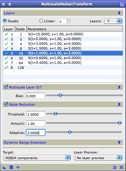
When using MMT for noise reduction, one generally needs to check the Noise Reduction box for each of the wavelet layers. Additionally, it seems that MMT noise reduction should be applied more strongly for the small-scale layers, and less strongly for the large-scale layers. (As near as I can tell, this seems to mean using larger Threshold settings on the smaller-scale layers, although for the life of me I don't know what the Threshold numbers mean.) After some iterating, I arrived at these settings:

These settings did manage to smooth the background, but I was left with a number of little dark blobs scattered around the image - I think you can see them here:

Hmm. Close, but no cigar. If only there were a way to get rid of those little dark blobs!


`Adaptive' to the rescue

Casting about for a solution, I read the long tooltip for the `Adaptive' sliders in the MMT noise-reduction dialog. It contained this line:  "Increase this parameter when you see isolated, high-contrast, relatively small structures that survive after finding an otherwise good noise threshhold value." This sounded promising. But how to minimize the time I'd have to spend iterating the Adaptive values?

Here's what I did: I used PI's ExtractWaveletLayers script to break the image down into its constituent layers of detail. Zooming in closely to each layer, I noticed that the `dark blobs' seemed to be about 16-32 pixels in size, roughly speaking. So, I gently increased the Adaptive settings for the 16-pixel and 32-pixel wavelet layers in MMT:

 Having done this, I got a better, smoother result:

It's a small victory, and I suppose it's nothing to brag about, but for a Pixinsight learner like me, it felt good to be able to smooth a noisy image this much, without the image looking too drastically over-smoothed. I was eventually able to use this noise reduction as one step in the overall processing of my Markarian's Chain image. That image will be the subject of the next post!

Globular Star Cluster M3

Harbinger of Summer - that's how I always think of the globular star cluster M3.

A little less than a hundred years ago, Harlow Shapley measured the distances to the globular clusters, and realized they form a spherical halo around a point that lies in the direction of the constellation Sagittarius. That was the beginning of the realization that our solar system is not at the center of the Milky Way galaxy. Globular clusters like M3 are classic summer objects; I've lost count of the number of times I've passed the short summer nights looking at them, through any number of different telescopes. Constellations like Sagittarius itself are rich hunting grounds for `globs' large and small, bright and dim. A trip to the southern hemisphere has, as one of its many treats, views of the huge, blazing Omega Centauri and 47 Tucanae globulars. Simply put, globular clusters are classic summer `eye candy'. Here's an image of M3 that I shot during the  June 2012 dark-moon cycle:

Globular star cluster M3
8-1/3 hours total exposure time
Evenly split between unbinned R, G, and B, shot in 4-minute subexposures.
Click the image for larger version, or click here for full size.

M3 will always have a special place in my astro-heart, since it was the first object I ever saw through a large amateur telescope. It occurred just over 10 years ago, in April of 2002. I went to one of my first Bay Area observing events, at a local hilltop site. I had my little 5" Meade ETX-125, and I was ready and excited to see some deep-sky objects! To my amazement, Bruce Jensen set up an 18" Starmaster dobsonian next to me. I'd never even looked at a telescope that big, at such close range, let alone looked through one. Bruce showed me M3, which was still rising in the east, and I was blown away. There was no going back - aperture fever took hold of me for good! (I'm lucky enough to be able to enjoy my own views through an 18" scope these days, something for which I'm very grateful, even if I'm mostly using my imaging rig these days.)

M3 is one of the farther-west of the bright globulars, so we see it in the (northern-hemisphere) spring, before the other globs are well-placed for viewing in the summer sky. I'll always associate M3 with April, May, and June, when we're enjoying the galaxies of Coma Berenices and Virgo, taking peeks at globs like M3 and M5, and dreaming of the summer Milky Way...

Acquisition and Processing

I shot the data for this image on three nights during the June 2012 dark-moon period, from the same site where Bruce Jensen showed me M3 through his Starmaster all those years ago. I decided to shoot unbinned R, G, and B images, to try and maximize the resolution of the image, and to avoid having to match the histogram of a luminance image to that of an RGB image. In the end, over the three sessions, I got about 36 four-minute subexposures through each filter. As with my other recent images, I used my Orion ED80 f/7.5 refractor on a Losmandy G-11 mount, with a short-tube 80 refractor and StarShoot camera for autoguiding. My trusty SBIG ST-8300 monochrome CCD camera gathered the photons, with a chip cooled to -15C.

Pixinsight processing followed my usual workflow, with deconvolution (i.e. sharpening) of the innermost core of the cluster, as well as smoothing of the background, done while the image was still linear. A wee touch of HDR Multiscale Transform helped to `un-blow-out' the cluster's core. I pumped up the color saturation in the brightest part of the cluster, so as to bring out the differences between the blue and orange stars.

Pixinsight geekery: The main thing I learned while processing this image was the usefulness of the `Amount' slider in Multiscale Medium Transform's noise-reduction routine. As with many of PI's tools, MMT is powerful yet somewhat hard to understand. I don't really know how to set the parameters for its noise-reduction routines, and I've always wanted to be able to increase the amount of noise reduction ever-so-slowly. Well, I should have guessed that the `Amount' sliders in the noise-reduction settings for each wavelet layer will do exactly that. I guessed at some Threshold values, starting with 4 for the first (1-pixel-scale) layer and decreasing roughly by half as I went from layer to layer. Then, having set those Threshold values, I set all of the Amount sliders to 0.1, and ran MMT. There was just the tiniest little bit of noise reduction in the background sky. (I used a luminance mask to protect the globular's stars.) By moving up the Amount sliders
one little increment at a time, I could get what I wanted: A nice, moderate amount of noise reduction.

Room for Improvement

I could have set the black point a little lower, to suppress the remaining background noise a little better. I could also have tried to dim/shrink the bright, burned-out-looking foreground stars. They're a little distracting. But, since the deep-sky object in question is a star cluster, I couldn't find a good way to make a star mask that didn't include stars from the cluster. So, I just left the stars alone and decided to post what I had. I think the thing I like the best about this image is the halo of very faint stars that makes up the outermost part of the cluster. I doubt I can see those visually, even through a large telescope. That's one of the joys of imaging, going deeper than the eye can see!

The M87 Chain and the Pixinsight Zone System

One of the greatest euphemisms in the world has to be the phrase `learning experience'. How often do we sugar-coat our mistakes by calling them `learning experiences'? I'm sure I've done it many times. This image provides an example, but in this case there's a bit more to it than that...

A portion of the Virgo galaxy cluster, with the giant elliptical galaxy M87 at top left, and part of `Markarian's Chain' of galaxies at right. Click the image for a larger version, or click here for full size.

Data Acquisition: Making the best of a bad situation

A few weeks ago, I was doing some backyard imaging, and the Virgo galaxy cluster seemed like the logical choice. Having shot a luminance image of the Leo Triplet not long before, I decided to do another one-night stand, with just luminance, but this time I wanted to shoot `Downtown Virgo'. (The origins of that term and its enthusiastic usage seem to go back to Jay Freeman and Jamie Dillon, two highly-accomplished Bay Area visual observers.) Specifically, I wanted to shoot the portion of the Virgo cluster called Markarian's Chain. It's a standard target, since it comprises a pretty, arc-ing chain of galaxies that stretch from M84 and M86 towards M88. Almost everyone works on an image of Markarian's Chain at some point. By planning it out in SkySafari Pro 3 on my iPad, I could see that if I rotated my camera just right, I could frame most of the chain pretty nicely on my ST-8300 sensor, using my ED80 f/7.5 refractor.

One thought nagged at me, though... What about conventions? As in sign conventions and angle conventions? Sky Safari Pro 3 has a really nice slider tool for rotating the position angle of one's field-of-view overlay, relative to the sky. This allowed me to plan my framing really easily. And when I'm imaging, I can download a frame from the camera, and use MaximDL to plate-solve it, which gives me the image's position angle on the sky. This is really handy, but.... what if these two pieces of software use different conventions for specifying the position angle? Hmm. I could wind up with a frame that's rotated 90 degrees from what I expect.

So, it wasn't a great shock when that's exactly what happened. Here's the framing I had planned on my iPad:

Here's how things actually worked out, since the two pieces of software treated the position angle differently:

Hrm. Rargh. What to do? I could have rotated my camera 90 degrees, but that would mean refocusing and probably re-doing the GOTO alignment. Given the couple of hours available for shooting Downtown Virgo before it went behind some trees, I didn't want to do that. So, I panned around in SSP 3 and looked for an alternative framing. Here's what I wound up with:

That seemed like the best compromise, since it caught part of Markarian's Chain, and included the giant elliptical galaxy M87, the real `heart' of the Virgo cluster. I shot a couple of hours of luminance (in 5-minute subexposures), and called it a night.

Processing: Pixinsight meets the Astro Zone System

A few weeks later, I had a little time to sit down with the data, and after using the very handy new preprocessing script in Pixinsight, I saw the following preliminary result (this is a closeup of two of the galaxies in the Chain):

Autostretched image of two galaxies in Markarian's Chain.

It's probably worth explaining what I mean by an `autostretched' image (also sometimes called an AutoSTF'ed image amongst Pixinsight enthusiasts). PI has a tool called `Screen Transfer Function' (STF), which stretches the brightness values of the image's pixels, solely for the purpose of displaying the image on the screen. It doesn't change the original pixel values in the image file, but it basically creates a temporary copy of the image to display on the screen, with the brightnesses changed so as to make the dim parts of the image more visible. The STF tool has a `Auto' button, which creates an image that nicely shows `what you got'. (I used one of these AutoSTF'ed images in my annotated Leo Triplet posting.) Such an image, though, usually doesn't make for a very pretty picture, since it shows just how noisy the dim background areas and dim parts of your target look. That graininess is a combination of instrumental noise and the eponymous photon shot noise (the latter coming from both the target objects and from the sky.)

At this point, my big goal was to do some noise reduction, and try to make the noisy, grainy-looking parts of the image look a little better. In this I was aided by Jordi Gallego's new presentation on noise reduction in PI. There's a lot of good information in this document, but I was particularly intrigued Jordi's slides 51 through 53, particularly #53. In this slide, he shows that one can make masks for applying different noise reduction settings to different parts of the image, such as:

• The dark background sky, which has the lowest signal-to-noise ratio (SNR), and is thus the `grainiest'-looking part of the image.
• The dim parts of the deep-sky object(s), which have fairly low SNRs, and thus mostly need smoothing and noise reduction.
• The bright parts of the deep-sky object(s), which have high SNRs, and thus can tolerate some sharpening, such as through deconvolution.

Aha! This is basically the same concept as Ron Wodaski's Astro Zone System. I borrowed a copy of this book from a fellow Bay Area observer a couple of years ago, and found it to be very interesting. Sadly, the book has been out of print for some time, but I was one of the lucky folks at the 2011 Advanced Imaging Conference who managed to get one of the copies Ron gave away. (Thanks, Ron!)

After a little fiddling around, I realized that PI's Range Selection tool works best on images that have already been stretched into a nonlinear state, so I made a copy of the image, applied its AutoSTF settings to Histogram Transformation, and applied that to the copy. I then used Range Selection on this stretched copy.

First, I made a mask that covered up the stars and galaxies, leaving only the dark background sky to work on:

After a little fiddling around, I stumbled on some settings in Multiscale Median Transform that smoothed the background reasonably well:

I was pleased with this result! It's not perfectly smooth, but I'm calling this a win, so far. Then, I made a mask for the `mid-SNR' zone, which included the fainter outer parts of the galaxies:

And then, by pulling back on my MMT noise reduction settings, I was able to smooth those areas somewhat. Next I made a mask to isolate the cores of the galaxies, for sharpening via Deconvolution:

After mid-SNR-range smoothing and high-SNR-range deconvolution, I had this image:

The brightness levels you see here are `Auto-STF' levels, and even with the noise reduction, they're not really good for posting on the web. So, since the image was still at a linear stage (i.e. not really brightness-stretched yet), it was time for a Histogram Transformation, some star shrinking, and a horizontal flip to match the correct appearance of this area on the sky:

Room for Improvement:

I think this was a good proof-of-concept project, for the Range Selection / `Pixinsight Zone System' approach. My masks could use some work, though. When I examine the image closely, I can see that some of the dim parts of the galaxies got left out of the masking process. Also, the various processing steps left an artificial ring around M87. There really are such things as ring galaxies, but M87 isn't one of them. I'm very interested in refining my touch with Range Selection, and to trying out the new Adaptive Stretch tool! A week or so after shooting these data, I managed to shoot Markarian's Chain with proper framing, and so we'll see how things go with this new data set.

Annotation Script - What did I capture in my image?

Here's another version of the Leo Triplet (luminance) image. This one has been overlaid with the results of Andres Pozo's plate-solving and annotation scripts. Thanks to Andres's hard work, I can take my image and `see what I captured':

The Leo Triplet, annotated. Click on the image for a larger version, or click here for full size.

Andres started a thread in the Pixinsight Forum back in March (see the link listed in the previous paragraph), and he's posted a number of updates to his scripts since the thread started. His scripts do two very useful things:

1) One script `plate-solves' the image. This basically means figuring what part of the sky has been captured in the image, and assigning a set of on-sky coordinates to each pixel in the image. (This is nicely described in Chapter 9 of Berry and Burnell.) By attaching metadata to the image (as part of something called the `FITS header'), the plate-solving script allows the annotation script to look at the image, and figure out the exact location (on the sky) of each pixel in the image.

2) The next script looks up objects in a set of online catalogues, and overlays symbols and coordinate lines on the image.

The whole thing is very slick, and after only one false start, I got Andres's scripts to work. The Annotation script overlaid the locations of objects from these three catalogues:

The Messier catalogue: This is a list of nebulous-looking objects in the sky, compiled by the 18th-century comet hunter Charles Messier. It's a list of roughly 100 bright deep-sky objects visible from mid-northern latitudes. The two big, bright galaxies in my image are Messier objects 65 and 66.

The NGC and IC catalogues: These catalogues were first compiled by J.L.E. Dreyer in the 19th century, and they list thousands of objects beyond the Messier catalogue. The great 18th-19th-century astronomer William Herschel found about 2500 of the objects that provided the initial `nucleus' of the NGC. Amazingly, Steve Gottlieb (a Bay Area observer) and others have been double-checking the NGC/IC catalogues visually!

The Principal Galaxy Catalogue: This list of about 70,000 galaxies was published by a group of French astronomers in the 1980s. Many of the faint `field galaxies' that an imager is likely to capture will turn out to have PGC designations.

Looking at my Leo Triplet image, it seems like I got pretty much all of the overlaid PGC galaxies. In other images that I've shot recently, about which more anon, the boundary between `what I got' and `what I couldn't get' occurs in the PGC galaxies. This isn't really surprising, since a large catalogue like the PGC includes objects that span a large range of apparent brightnesses. If I had more time, it would be interesting to compile lists of the PGC galaxies that I did and didn't get, so as to characterize the depth of my image. How deep can a 3-inch f/7.5 refractor with an amateur CCD camera go in a night or two? Andres's script offers a way of estimating this.

I'm pleasantly surprised at how much I enjoy looking at the image with the annotation overlays. They give me a sense of what's in this part of the sky, and somehow they add depth and richness to the image. Naturally, the `pretty picture' version of an image probably shouldn't have annotations like this on it, but it's nice to be able to make an annotated version easily. The two versions complement each other, I think.

The (Leo) Luminance Triplet

For such a dry winter, California didn't have a lot of imaging-quality skies in early 2012. We had some late-season rain and mountain snow, which was good for our hydro balance, but not so good for the spring galaxy season. I finally got out in mid-May, and spent a couple of nights shooting M65, M66, and NGC 3628, otherwise known as the Leo Triplet. Here's the result, sized for a 15" MacBook Pro screen:

This is what's known as a `luminance' image, which means it was shot with a black-and-white (or `monochrome') CCD camera, through a clear (or `luminance') filter. In order to make a color image, I'll need to shoot it through 2 or 3 color filters. If all goes well, I hope to shoot it through Red, Green, and Blue filters before the spring season slips away. The subexposures for this image were each 5 minutes long, and I shot about 50 of them over two nights, for a total exposure time of about 4 hours. As always, the imaging scope was an Orion ED80 f/7.5 semi-apo refractor.

This was also the inaugural imaging run for my new (to me) Losmandy G-11 mount. I got a great deal on it from a fellow Bay Area imager, and I spent the April dark-moon period learning some of the ins and outs. I feel like I can polar align, acquire targets with the Gemini 1 (Level 4) goto system, and I can get pretty good autoguiding. During the nights when I shot these luminance frames, the RMS error on my guider corrections was running about 1/2 pixel in both RA and Dec.

I processed this image in Pixinsight, making use of the new Batch Preprocessing script. Very handy! Many thanks to the folks who wrote that script. Also many thanks to Mike Schuster for writing the PSF Estimation script, which auto-picked hundreds of stars and gave me the parameters of the point-spread function, which I used for Richardson-Lucy deconvolution. (Deconvolution is a sharpening routine that I used to bring out some of the details in the galaxies.) The hardest part of the whole processing workflow was the noise reduction, which I did with Multiscale Median Transform. Once I had the noise somewhat beaten down, I could get a halfway-decent stretched image from the Histogram Transformation. I did a bit of HDR Median Transform, but not nearly as much as I might use on, say, a large bright nebula.

I hope to be able to get out and shoot some RGB color data if I'm lucky; it would be nice to add color to these galaxies!

The Orion nebula: Reworking some year-old data

If you've not yet had the opportunity to look at M42, the great Orion nebula, through a telescope, you owe it to yourself to try and find an opportunity to do so. Even though today's entry is part of an `imaging blog', M42 is the kind of object that's beautiful any way you look at it. As long as you've got a clear sky, and are (hopefully) away from city lights, you can see this nearby star-forming complex in some way, regardless of the gear you've got.

I just now spent a moony evening reworking some unbinned R, G, and B data that I shot about a year ago. Every winter, it's the same old routine: Try to get some decent data on M42. Something always gets in the way, though. In early 2011, it was bad weather and camera issues... a story for another time. I managed to shoot some unbinned L, R, G, and B data, but not a heck of a lot. To the best of my memory, the data for this image don't amount to much more than several hours total. Since it's now February, and I'm not 100% sure if I'll get in a decent M42 dataset in 2012, I thought I'd fool around with this old stuff from last year. See if I could make something semi-presentable.

After an evening spent in front of the computer, I happened to go outside, and as I was walking back in, I looked up, and there he was: Orion, the hunter. The constellation was just passing across the meridian, with the bright gibbous moon due north of it. Even with lights in my eyes, and under a city sky, I could make out the bright stars that delineate the pattern: Betelgeuse, Rigel, Bellatrix, Saiph, Alnitak, Alnilam, Mintaka. And there was the sword of Orion, with the middle `star' being M42. This object is so bright that it (or at least the stars in and around it) can be seen under almost any sky, it seems.

Unlike most deep-sky objects, M42 is worth looking at with virtually any optical instrument. The belt and sword of Orion are great in binoculars. Small telescopes show the nebulosity. Large telescopes under dark skies provide one of the few `imaging-like' experiences in visual observing. A greenish color can even be seen in the brightest part of the nebula, in a big scope. The details just go on for days and days.

As an imaging project, M42 presents an almost limitless field of challenges and rewards. With modest equipment and short exposures, one can still get something. Advanced imagers have gotten some incredible results.

Processing in Pixinsight:

This image certainly isn't incredible, but I'm glad that I was able to squeeze a bit of detail out of such data as I had. I spent a fair amount of time on this in Pixinsight, and eventually I gave up on trying to combine the luminance data with the color data. Both my RGB image and my Luminance image were the result of high-dynamic range combinations, for which I'd shot long- and short-exposure frames. Matching the histogram from the L image to the histogram from the RGB image seemed to be taking forever, with little end in sight. I bailed and just went for the RGB.

Getting a good color balance was really tricky, and I just couldn't get it quite right. The stars in the linear image had all sorts of blue and cyan issues, and by the time I got them to look semi-normal, the blue color in the nebula was pretty well gone. I could have (and should have) worked that problem harder, but since this was a `let's see what we can get out of this stuff without too much struggle' project, I didn't sweat it that hard.

I did a bit of Richardson-Lucy deconvolution while the image was still linear, but nothing drastic. I would have liked to have gotten a better sharpening result, but I found that I kept getting bright `wormy' artifacts if I wasn't careful. I think that a really good deconvolution would be pretty substantial project, even with the help of Dynamic PSF.

After histogram stretching, I had to spend a fair amount of time finding the right parameters for an application of HDR Multiscale Transform, to knock down the over-brightness of the area around the Trapezium. Once I got that area tamed, it was rather washed out, as usual. Some additional luminance masking and an extra saturation boost in that area helped a bit, although it left some purple haze around the Trapezium stars.

There's plenty of room for improvement in this image, but I'm glad that I can at least post some sort of M42 image. I hardly feel like `an imager' without one. With a little luck, maybe I can finally get a decent set of data later this month and in March. It would be nice to really go deep on this thing, and under good seeing. We'll see how it goes!

As per usual, there's an amazing image of the object from the Hubble Space Telescope.

Eagle nebula in B&W H-alpha

Ever since this summer's imaging session at Lassen, I've wanted to process the hydrogen-alpha data that I acquired as a black-and-white image. I spent this evening working on the data in Pixinsight, and here's what I've come up with so far:

Acquisition:

I shot these data during two nights, using 15-minute subexposures through an Astrodon 3nm H-alpha filter, for a total exposure time of 5 hours. This was with the 80mm refractor and borrowed QSI camera that I described in a previous post.

I've always enjoyed the look of black-and-white hydrogen-alpha images, and I wanted to try and make one myself. Images like this remind me of the days of heroic long exposures on gas-hypered Technical Pan 2415 film... days that I have to admit I didn't experience first-hand. And, frankly, I'm not too sorry about it, although it would make for some nice bragging rights. Me, I'm grateful for CCD cameras and autoguiders, which make the whole thing a lot more do-able, although it's still a fair amount of work.

The real key to an image like this is the narrowband hydrogen-alpha filter. I'm lucky that my friend from Cilice, who loaned me the camera, had invested in a filter with such a narrow bandpass. Besides bringing out all of the lovely emission nebulosity (which would look deep red in a color image), a filter like this makes the stars look very small! That's a very nice `perk', although it makes focusing and framing the image rather time-consuming. No need to shrink the stars in software when you have such tiny stars to begin with! I can't wait to get an H-alpha filter for my SBIG filter wheel, someday. I think I'll go with 3nm - it's worth the extra effort.

Processing in Pixinsight:

Like most CCD image processing, part of my workflow happened while the image was still linear, and then I took it to the non-linear realm with a histogram stretch, where I did further processing.

I started by using the A Trous Wavelet Transform (ATWT) tool to reduce noise, following the example from Juan Conejero's `tutorial post'. I used considerably less aggressive ATWT noise-reduction settings than Juan's example, though. Then I did some Richardson-Lucy deconvolution, again following a tutorial-like post by Juan. A real key to getting Deconvolution to work is the use of Dynamic PSF to model the telescope's point-spread function.

Once I had reduced noise with ATWT and applied a bit of deconvolution, I stretched the image into the non-linear realm using Histogram Transformation. (I just applied the stretch parameters from an AutoSTF into HistoTrans.) As per usual Pixinsight practice, I used the HDR Multiscale Median Transform (formerly HDRWT) to bring down the brightness in the central part of the nebula. I found that increasing the number of wavelet layers to 8 helped bring out detail nicely, and did the best job of `taming' the brightest areas. I did another moderate histogram stretch to increase contrast, and then applied the Local Histogram Equalization (LHE) tool, with a contrast limit of 2.0 and and Amount of .25.

A last, light little shot of ACDR was the last step. I did this with the built-in lightness mask enabled, so as to apply it only to the darkest areas. These areas had had their noise increased a bit by LHE.

Assessment:

I'm reasonably pleased with how this image turned out. I like the way the deconvolution brought out detail around the `Pillars of Creation' and other dusty structures in the nebula. HDRMMT also helped to bring out a fair amount of detail, and LHE pumped up the contrast between adjacent light and dark areas.

Naturally, I'd love to get additional hours of data, to bring out even more nebulosity at a reasonably high signal-to-noise ratio. Maybe next summer!

Oh, I almost forgot: I flipped the image left-for-right, compared to my previous Eagle nebula image. I hadn't realized that the previous image was oriented incorrectly. I think this one matches the published `Pillars' images better.

Hmmm... I wonder... since LRGB combinations in Pixinsight are supposed to be assembled from non-linear images, I wonder if I could get the histogram of the RGB image into the right kind of shape to match this one, and use this B&W H-alpha image as the luminance for an LRGB combine?  Hmm... I ought to check that out.

M31 2011

A major event for California observers is the yearly California Star Party, or `Calstar'. My Bay Area buddies and I look forward to it each year. In 2011, I worked on M31, the Andromeda galaxy. M31 is a classic autumn object, rising in the evening and riding high for much of the night. I'd spent previous Calstars observing it in detail visually, and this year I wanted to get the best possible RGB imaging data that I could.

Happily, I'd just taken delivery of a new SBIG ST-8300M CCD camera, and I was eager to try it out. (Many thanks to Sam Sweiss at Scope City for helping me get it! This also meant that I could give the QSI 583 back to my Cilice friend, enabling him to image at Calstar.)

SBIG ST-8300M and Orion 2" LRGB filter wheel

Like the Lassen run in which I imaged the Eagle nebula, this year's Calstar was blessed with good weather. I got in a solid 3 nights of clear, dark skies, and managed to get several hours each of unbinned R, G, and B images. Calibration, integration, and processing in Pixinsight gave me this image:

The Andromeda galaxy (M31), approx. 15 hours total exposure time

After talking about star shrinking in yesterday's blog entry, I went back to RBA's M31 star-shrinking tutorial, and worked the problem some more. The image above has had its `medium-sized' stars dimmed, following Rogelio's tutorial. As he pointed out, M31 is not in the plane of the Milky Way, and thus doesn't need a lot of star reduction, but I think it helps the overall appearance of the image.


Room for Improvement:

I'm fairly pleased with the star shrinking / reduction / whatever you want to call it, but I need to double-check that I haven't affected the starlike nuclei of M31, M32, and NGC 205 too much. I also really want to figure out how to reduce the brightest and most bloated stars, like the blue one that appears to the lower left of M32, and the orange one that appears to the upper left of M32. As I stretched the image, these got so big, their halos make them look like `candidate satellite galaxies'. I still haven't figured out how to make a star mask that isolates only the brightest stars.

Eagle nebula 2011

One can't very well have an `imaging blog' without eventually posting some images. Here's the first image I think is good enough to be worth putting out there. This is Messier object 16 (`M16'), the Eagle nebula. I shot these data in the summer of 2011, from a trailhead parking lot in Lassen Volcanic National Park, California.

If I feel the image supports it, I like to make three crops:

1440 x 900 (15" MacBook Pro)
1200 x 800 (13" MacBook)
1024 x 768 (iPad and many older monitors)

I'm a Blogger newbie, so I'm still trying to figure out how to provide links to all three sizes, in a way that's convenient for the reader.

Acquiring the data:

I shot this image during the late July / early August dark-moon cycle, from a site at about   8200 feet (2500 meters) above sea-level. (It's silly, but I sometimes like to point out that it's about as high as ESO's Paranal observatory in Chile.) Being able to image from a dark, isolated site at a reasonably high altitude is really helpful for building signal-to-noise ratio in one's image. Under those conditions, there is very little light pollution contributing to the photon shot noise, so most of that noise just comes from scattered starlight in the Earth's atmosphere, the Earth's natural airglow, dust in the plane of the solar system, and the intergalactic background light. (See Brian Skiff's articles on the night sky background, nicely organized and hosted on Jerry Lodriguss's site, for a nice explanation of why the night sky isn't perfectly black.) In addition to the dark sky, the chilly nighttime temperatures make it easier for the camera's Peltier cooler to keep the CCD chip reasonably cold. (I shot these data at -20 degrees C.)

This Lassen session was blessed with excellent weather - I basically had 8 clear nights in a row. This allowed me to capture multiple hours through each color filter. This image was made from unbinned R, G, B, and H-alpha data. I shot Luminance data, but didn't use it in the processing for this version.

For this session, I was using my telescope (an Orion ED80 semi-apochromatic refractor on an Orion `Sirius' mount), while borrowing a QSI 583 CCD camera from my friend at Cilice Astrophotography. Here's the setup I was using at the time:

Processing:

If I have the time and energy to do much with this blog as time goes by, I'll hopefully have a lot more to say about Pixinsight, the software that I used to make the image. I've bee sufficiently impressed with the work that's been done by Pixinsight users - especially the many APODs from RBA - that I decided to try and learn the software. This isn't an easy task, as I've discovered! The story of the Pixinsight learning curve will, hopefully, be a big part of what I'll describe in this blog, if I have the time.

For this image, I did the following things in Pixinsight:

1) Calibration and stacking of the raw CCD images. (See, for example, Vicent Peris's tutorial on master calibration frames, Jordi Gallego's PowerPoint presentation on image integration, and the new Pixinsight reference documentation on image integration.)

2) Dynamic Background Extraction (DBE) for each of the R, G, and B channels, RGB combination, Background Neutralization, and Color Calibration. (See, for example, the new instructional video that walks the viewer through these tasks, as well as Harry Page's excellent set of video tutorials.)

3) While still at the linear stage, I used the A Trous Wavelet Transform tool to reduce background noise, following Juan Conejero's example.

4) Histogram Transformation to stretch the image from the linear domain (and thus largely invisible on-screen) to a brighter, more visible version.

5) Saturation of the red M16 nebulosity.

6) Reduction of green color noise with the Selective Color Noise Reduction tool.

7) Star shrinking (with Morphological Transformation) and star desaturation.

Room for improvement:

The unfortunate thing about being `an imager' is that when I look at my images, I can only see the deficiencies! There's a lot about this image that I'd like to improve, and hopefully my Pixinsight skills will one day improve to the point where I can make those improvements.

The main thing I'd like to change about the image is the `star carpet'. This is a real problem for objects in the plane of the Milky Way. There are so many stars in our galaxy's disk that it's nearly impossible to shoot something like a Messier object in the MW plane without the field being full of stars. As one stretches the nebulosity, the stars get stretched, too, until they become bright enough to dominate the field, rendering the details of the nebulosity less visible.

I'd like to reduce the distracting effect of the `star carpet', and I'm trying to learn some techniques to help me do that. These include RBA's tutorial on star shrinking, and Vicent's recent NGC 7023 tutorial. Hopefully one day I'll be able to post another version of this image with fewer distracting foreground stars!